Installing a new ESRI extension Failture (Registration Failed)

 Installing a new ESRI extension Failture (Registration Failed)

 

This error appear when installing a new extension on ArcGIS desktop environment 10.x.

To fix run as Administrator. 

 

 

If you are running ESRIRegAsm.exe manually, run the Command prompt (cmd) as administrator.

Executing tools in ModelBuilder

Executing tools in ModelBuilder

 

This tutorial takes you step-by-step through creating a model and executing tools in ModelBuilder. You start by adding a tool to ModelBuilder and supplying values for the tool's parameters. This constructs a process. A model is built by connecting processes.

This tutorial builds a very simple model that identifies the vegetation types near proposed roads. In the model, the roads are first buffered using values from a distance field in the roads attribute table. The output from the Buffer tool is used to clip the vegetation data to create a dataset of vegetation types within the buffer polygons.

The tutorial is composed of six broad steps:

Steps:

1. Copy tutorial data
2. Open the map document
3. Create a new model
4. Add tools and data to the model
5. Fill in the tool parameters
6. Run the model
7. Save the model

1—Copying tutorial data

It is assumed that you have installed ArcGIS Desktop (ArcView, ArcEditor, or ArcInfo) before you begin this tutorial. The data required for this tutorial (included on the ArcGIS Desktop CD) by default is installed in C:\arcgis\ArcTutor. The tutorial scenario is fictitious, and the original data has been adapted for the tutorial.

Steps:

1. To avoid corrupting the original data, copy the ModelBuilder folder from C:\arcgis\ArcTutor to the C drive on your computer. If you are copying the data to another drive or location, make sure to use that location for all the steps below.

2—Opening the map document

Browse to the C:\ModelBuilder folder in Windows Explorer and double click the Extract Vegetation.mxd. This will start ArcMap and open the map document, or

Steps:

1. Start ArcMap by clicking Start > All Programs > ArcGIS > ArcMap 10.
2. On the ArcMap - Getting Started dialog box, click Existing Maps > Browse for more.
   The Open ArcMap Document dialog box appears.
3. Browse to C:\ModelBuilder folder, select Extract Vegetation.mxd, and click Open.
   This opens the Extract Vegetation.mxd.

3—Creating a new model

Steps:

1. Click the ModelBuilder button on the ArcMap Standard toolbar.
   This opens the ModelBuilder window for editing.
You can also create a new model by right-clicking an existing toolbox and choosing New > Model. This creates a model in the toolbox with a default name and opens the model for editing.

4—Adding tools and data to a model

Now that the model is open for editing, you will add two tools using the Search window:

Steps:

1. In ArcMap, click Geoprocessing > Search For Tools.
   This opens a Search window that you can dock anywhere in ArcMap.

   
   
2. On the Search window, type Buffer, then click the Search button .
   The Buffer tool is listed along with other search items.
3. Drag the search item Buffer (Analysis) (which represents the Buffer tool found in the Analysis toolbox) onto the ModelBuilder canvas in the white space.
   This adds the tool and the output data variable to the model. The output variable is connected to the tool by a connector. Both the tool and output data are empty (without color) as none of the tool parameters have been supplied.
4. Search for and add the Clip tool in the Analysis toolbox in a similar manner. If the two tools overlap, click the Auto Layout button on the ModelBuilder toolbar to arrange the tools.
There are two other methods to add tools in a model that are not used in this tutorial, but have been listed to introduce you to them:
• In the Catalog window, navigate to Toolboxes > System Toolboxes > Analysis Tools > Proximity. You can select Buffer and drag the tool onto the ModelBuilder canvas in the white space.
• On the ModelBuilder Standard toolbar you can click the Add Data or Tool button , and navigate to Toolboxes > System Toolboxes > Analysis Tools > Proximity. Select the Buffer tool and click Add.

5—Filling in tool parameters

Now that the tools are added to the model, you will fill in the tool parameters.

Steps:

1. In ModelBuilder, double-click the Buffer tool to open its tool dialog box.
2. For the Input Features parameter, click the browse button and navigate to the input geodatabase (C:\ModelBuilder\ToolData\Input.gdb).
3. Choose the PlanA_Roads feature class and click Add.
4. Once you fill in the input features, the Output Feature Class parameter is automatically generated and filled in for you. Replace this autogenerated output name by clicking the Browse button for the Output Feature Class parameter. Navigate to the output geodatabase in the ModelBuilder folder (C:\ModelBuilder\Scratch\Output.gdb), type BufferedFC for the output name, then click Save.
5. For the Distance parameter, choose the Field option and choose the Distance field from the drop-down list.
6. Click OK. (You don't need to fill in any other parameters.)
   The input data is added as a variable to the model (the blue oval in the above illustration) and is automatically connected to the Buffer. The input variable (the blue oval), the tool (the yellow rectangle), and the output variable (the green oval) change colors to indicate that all parameter values have been supplied and the tool is ready to run. Note that clicking OK on the tool dialog box does not execute the tool in ModelBuilder.

   When data or tools are added to a model, they are referred to as model elements. There are three basic types of elements: variables (such as datasets), tools, and connectors.
7. Now double-click Clip to open its tool dialog box.
8. For the Input Features parameter, click the Browse button and navigate to the input geodatabase (C:\ModelBuilder\ToolData\Input.gdb).
9. Choose the vegtype feature class and click Add.
10. For the Clip Feature parameter, click the arrow and choose BufferedFC from the drop down list. The blue recycle symbol means that BufferedFC is a variable in the model. This variable was created in the model when you added the Buffer tool.
11. Click the browse button for the Output Feature Class parameter, navigate to the output geodatabase (C:\ModelBuilder\Scratch\Output.gdb), type ClippedFC for the dataset name, then click Save.
12. Click OK on the Clip tool dialog box.
    The output variable of the Buffer tool is automatically connected (using a connector) as an input to Clip, as illustrated below.

    
    

6—Running the model

After all the parameters of the tools have been filled in, the model is ready to run.

Steps:

1. Before you run the model, select the ClippedFC variable, right-click, then click the Add To Display option. Setting this option ensures that when the model is run from ModelBuilder, the output ClippedFC will be added to the display in ArcMap for quick viewing of the results.
2. From the ModelBuilder menu, click Model > Run Entire Model.
   The model runs and the output is added to the display. After the model has finished running, both the tools (the yellow rectangles) and output variables (the green ovals) show a drop shadow around them indicating that these tools have been run.

Running the model on different roads

To run the model on different roads (such as PlanB or PlanC feature classes), you have two choices:

1. Double-click Buffer and navigate to another feature class, or
2. Drag the data from the Catalog window onto the ModelBuilder canvas to create a new data variable, then connect this variable to Buffer. Follow the steps below to see how this works.

Steps:

1. On the ArcMap menu, select Geoprocessing > Geoprocessing Options.
   1. Ensure that the check box next to When connecting elements, display valid parameters when more than one is available is checked.
   2. Click OK.
2. Navigate to the input geodatabase in the Catalog window.
3. Choose the PlanB_Roads feature class and drag it onto the ModelBuilder canvas.
4. Click the Connect button , then do the following:
   1. Click the PlanB_Roads variable element.
   2. Click the Buffer tool element. A shortcut menu appears containing the choices of available parameters for the tool.
   3. Choose the Input Features parameter from the list.
   This connects the PlanB_Roads variable to Buffer and automatically disconnects the PlanA_Roads variable that was previously connected to the tool. The model elements lose their drop shadow, signifying that the model has not been run with the new variable you added.
5. Double-click Buffer and choose the correct distance field from the PlanB_Roads feature class.
6. Run the model with Model > Run Entire Model.
   The model runs and the output is added to the display. After the model has finished running, both the tools and output variables show a drop shadow around them indicating that these tools have been run. The existing output ClippedFC layer (from the previous run with PlanA_Roads) in the ArcMap table of contents is updated with the results from PlanB_Roads.

7—Saving a model

Saving is the last step for this tutorial. You will use the saved model in the Creating tools with ModelBuilder tutorial.

Steps:

1. Click the Save tool on the ModelBuilder toolbar and navigate to C:\ModelBuilder.
2. A model can only be saved in a toolbox. Click the New Toolbox icon on the navigation window.
   A toolbox with a default name is added in the workspace.
3. Change the name to MyTools.tbx.
4. Select MyTools.tbx and click Save to save the model with the default name (Model).

Additional analysis

If you want to do some analysis with the model, you can add the Summary Statistics tool to get a summary table of affected area by vegetation type within the buffer polygons around the proposed roads.

Steps:

1. Use PlanA_Roads as input in the Buffer tool for this analysis.
2. Find the Summary Statistics tool in the Search window.
3. Drag the tool into the model.
4. Double-click the Summary Statistics element to open the tool dialog box.
5. For the Input Table parameter, click the arrow and choose ClippedFC with a blue recycle icon next to it from the drop down list. This recycle icon means it is a variable in the model.
6. For the Output Table parameter, browse to the output geodatabase (C:\ModelBuilder\Scratch\Output.gdb), type AffectedVegetation for the name, then click Save.
7. For the Statistic Field(s) parameter, choose Shape_Area from the list.
8. Click the cell next to Shape_Area under Statistic Type and choose SUM from the drop down list.
9. For the Case field parameter, choose VEG_TYPE from the list.
   The completed Summary Statistics dialog box is illustrated below.
10. Click OK.
11. Confirm that the Add to Display option is checked for ClippedFC by right clicking it.
12. Right click and check the Add to Display option for the AffectedVegetation variable. This will add the ouput to the display after the model runs.
13. Run the model.
    The output ClippedFC and the AffectedVagetation table is added to display in the ArcMap table of contents.
14. Open the table by right-clicking and clicking Open.
    The table shows a summary of area by vegetation type within the buffer polygons that will be affected by the proposed roads for plan A.

Copyright © 1995-2011 Esri. All rights reserved.

Creating tools with ModelBuilder

Tutorial: Creating tools with ModelBuilder

 

This tutorial takes you step-by-step through the process of creating a model tool. In this tutorial, the model built in the Executing tools in ModelBuilder tutorial is made into a useful tool by exposing model variables as model parameters.

For a broad overview of creating model tools, see A quick tour of creating tools with ModelBuilder.

It is assumed that you have installed ArcGIS Desktop (ArcView, ArcEditor, or ArcInfo) before you begin this tutorial. The data required for this tutorial (included on the ArcGIS Desktop CD) by default is installed in C:\arcgis\ArcTutor. The tutorial scenario is fictitious, and the original data has been adapted for the tutorial.

To avoid corrupting the original data, copy the ModelBuilder folder from C:\arcgis\ArcTutor to the C drive on your computer. If you are copying the data to another drive or location, make sure to use that drive for all the steps below.

Steps:

1. Open the map document.
2. Create the model.
3. Expose tool parameters.
4. Create model parameters.
5. Rename model elements.
6. Set model parameter order.
7. Set model parameter type.
8. Set filters on model parameters.
9. Set symbology for output data.
10. Manage intermediate data.
11. Change general model properties.
12. Document the model.

1-Open the map document

Browse to the C:\ModelBuilder folder in Windows Explorer and double click the Extract Vegetation.mxd. This will start ArcMap and open the map document, or

Steps:

1. Start ArcMap by clicking Start > All Programs > ArcGIS > ArcMap 10.
2. On the ArcMap - Getting Started dialog box, click Existing Maps > Browse for more.
   The Open ArcMap Document dialog box appears.
3. Browse to C:\ModelBuilder folder, select Extract Vegetation.mxd, and click Open.
   This opens the Extract Vegetation.mxd.

2-Creating the initial model

Follow the steps in Executing tools in ModelBuilder. The same model is used in this tutorial as the starting point.

If the model was saved previously, open the model by right-clicking the model and selecting Edit. If this model was saved after the model was run in the "Executing tools in ModelBuilder tutorial," the model elements may have a drop shadow around them. To remove the drop shadows, validate the entire model by clicking the Validate Entire Model button on the ModelBuilder toolbar.

Double-click the example model from the Catalog window. The tool dialog box opens but shows no parameters, as illustrated below.

If you run the tool by clicking OK, the model will run. The output of the model (ClippedFC) will not be added to the ArcMap table of contents, even though Add To Display was checked for the output variable. The reason is that when a model is run from its tool dialog box, the Add To Display setting is ignored. To add the output to the display, you must make the output variable a model parameter.

Another reason for creating model parameters is that you want to run the model with different inputs without having to open ModelBuilder every time, as illustrated below.

Once the model parameters have been created, you can execute the model from its tool dialog box, supplying different values for the Input Roads, Buffer Distance, Input Vegetation, Output Clipped Feature Class, and XY Tolerance parameters. You don't have to open ModelBuilder each time you want to run the model—you can use the tool dialog box instead. An added advantage of running a model from its tool dialog box is that a result in the Results window is created; running a model within ModelBuilder does not create a result in the Results window.

The remaining steps will expose model variables as parameters so they appear on the model tool dialog box as shown above.

3-Exposing tool parameters

To define the Buffer Distance and XY Tolerance parameters, you need to create model variables for them.

When you add a tool to a model, model variables are automatically created for input and output datasets, but not for any other tool parameters. The reason is aesthetics—if variables were automatically created for every tool parameter, the model diagram would quickly become unreadable. For example, when you add the Buffer tool to a model, a variable is automatically made for the Output Feature Class parameter. After you right-click Buffer and fill in the Input Features parameter, a model variable is created for the input features. All other parameters, such as Distance, Side Type, and End Type, are not automatically added as variables in the model. The steps below create model variables for Distance [value or field] and XY Tolerance.

Steps:

1. In the Catalog window, right-click the model and click Edit. This opens the model in ModelBuilder.
2. Right-click Buffer.
3. Click Make Variable > From Parameter > Distance [value or field].
   This adds the Distance parameter as a variable in the model.

   
   
4. Right-click Clip.
5. Click Make Variable > From Parameter > XY Tolerance.

4-Creating model parameters

Now that you've created variables for Distance and XY Tolerance, you're ready to make model parameters.

Steps:

1. Right-click Distance [value or field] and check the Make Parameter option, as illustrated below.
   The letter P appears beside the variable, indicating it is a model parameter. This model parameter then also appears on the model tool dialog box.
2. Create model parameters for the following variables (do not make a model parameter for BufferedFC):
   • PlanA_Roads
   • vegetype
   • XY Tolerance
   • ClippedFC

5-Renaming model elements

ModelBuilder assigns default names to variables. Variable names are used for parameter names on the model tool dialog box. It is good practice to rename variables, especially if they are model parameters.

Steps:

1. Right-click PlanA_Roads and click Rename.
2. Type Input Roads and click OK.
   The name of the variable changes to Input Roads.
3. Rename the remaining variables as follows:
   • Rename Distance [value or field] to Buffer Distance.
   • Rename vegetype to Input Vegetation.
   • Rename ClippedFC to Output Clipped Feature Class.
4. Save the model. You do not need to exit ModelBuilder.
5. Double-click the model from the Catalog window to open the model tool dialog box. You may have to move or minimize the ModelBuilder window to access the Catalog window. The model tool dialog box should look similar to the illustration below. The order of the parameters may be different on your dialog box, but this is not an issue since you'll change the order below.
   You can execute your tool by clicking OK, but it is suggested that you choose a different output feature class before executing. The tool executes, and the output feature class is added to the ArcMap table of contents. Unlike running a model within ModelBuilder, running the model from its dialog box does not change the model diagram.

6-Setting model parameter order

As illustrated above, the order of the parameters is not ideal. The standard practice is to order parameters as follows:

• Required input datasets
• Other required parameters that affect tool execution
• Required output datasets
• Optional parameters

Steps:

1. In ModelBuilder, click Model > Model Properties.
2. Click the Parameters tab.
3. Choose the Input Roads parameter and move it to the top using the Up and Down arrow buttons on the right side.
4. Change the position of other parameters as shown below:

7-Setting model parameter type

Once the model parameters are set in the correct order, change the type of the parameter. If a parameter is a required parameter of a tool in the model, you will not be able to change the type to optional from these settings.

Steps:

1. In ModelBuilder, click Model > Model Properties.
2. Click the Parameters tab.
3. Click the cell under the Type category for XY Tolerance. A list appears with two options. For this example, keep XY Tolerance as an optional parameter and the rest as a required parameter type as shown in the illustration below.

8-Setting filters on model parameters

You can restrict the type of input to any parameter by applying filters to parameters. The model in this example expects the Input Roads parameter to be line features. In the following steps, the parameter is modified by applying a filter so that it only accepts line features.

Steps:

1. Click Model > Model Properties.
2. Click the Parameters tab.
3. Choose Input Roads and click the cell under the Filter category.
4. Choose the Feature Class filter.
   The Feature Class dialog box opens.
5. Uncheck all the types except Polyline and click OK.
6. Click OK on the Model Properties dialog box to apply the filter.

9-Setting symbology for output data

The output of a model can be set to have a particular symbology that is used to display the output. For this example, the symbology is based on the type of vegetation within the buffer zone. To set the symbology for the output data, the first step is to create a layer file, and the second step is to define the layer file in the output data properties. For this tutorial, a layer symbology file has been created for you.

Steps:

1. In the ModelBuilder window, right-click Output Clipped Feature Class and click Properties.
2. Click the Layer Symbology tab.
3. Browse the layer file from the ToolData folder that you copied in C:\ModelBuilder\ToolData.
4. Choose OutputSymbology.lyr and click Add.
5. Click OK.

Learn more about creating a layer symbology file

10-Managing intermediate data

When you run a model, output data is created for each process in the model. Some of the data created is of no use after the model is run since it was only created to connect to another process that creates new output. Such data is called intermediate data. All outputs except the final output, or those that have been made model parameters, are automatically made intermediate data in the model. In this example, the output of the Buffer tool is only useful as an input to the Clip tool and is not used after that, so the Intermediate option is checked. You can choose to save the intermediate data by unchecking the Intermediate option.

11-Changing general model properties

You can set the model name, label, and description for the model.

Steps:

1. Click Model > Model Properties from the ModelBuilder interface.
2. Type ExtractVegetationforProposedRoads for the name of the model. No spaces are allowed in the model name.
3. Type Extract Vegetation for Proposed Roads in the Label text box. Spaces are allowed in the model label. This label is used to display the model name in the Catalog window.
4. Type the desired text in the Description text box.
   Check the Store relative path names (instead of absolute paths) option so that you can share your model tool or move your model data and model to a different location. This option is not used in this tutorial but has been introduced here as a good practice to follow for your future models and model tools that you will share.

   Learn more about the relative path option
5. Click OK.
   
   
6. Save the finished model and exit ModelBuilder.
Double-click the model from the Catalog window to open the model tool dialog box. Since the model was saved with the predefined values, all the parameters on the dialog box are filled in. You can change the value of any parameter here by entering a new value. Click OK to run. The final output of the model (Output Clipped Feature Class) is added to the display by default, and the model messages are posted in the Results window. To see your results, uncheck the Vegetation Type layer in the map document table of contents.

12-Documenting the model

It is always a good practice to document the model before you share it. To document:

Steps:

1. Right click the model in Catalog window and click Item Description.
   This opens the Item Descriptionwindow, displaying the Description page.
2. Click the Edit button on the Item Description window
   This opens the documentation editor to enter the item description.
3. Type in appropriate description for each item in this model and click the Save button.
To learn more about documenting take A quick tour of documenting tools and toolboxes

Additional analysis

If you want to do some analysis with the model, you can add the Summary Statistics tool to get a summary table of affected area by vegetation type within the buffer polygons around the proposed roads.

The steps below will also show you how to use a model as a tool inside another model.

Steps:

1. Open a new model by clicking the ModelBuilder button on the ArcMap Standard toolbar.
2. Now that you have created a model tool, you can use it just like any other tool. You can add the model tool to a new model by dragging it from the Catalog window into the new model, as illustrated below.
Since the model tool had predefined values for input and output parameters, it is added to the new model with input and output variables (the blue and green ovals). Note that not all parameters of the model tool are exposed when added in another model. Also, the original names of the input datasets have been used. You can make variables and rename them as described earlier in this tutorial.
3. Open the Search window (if not already open in ArcMap) by clicking Geoprocessing > Search For Tools.
   This opens the Search window.
4. In the Search window, type Summary Statistics and click the Search button .
5. Drag the tool into the model.
6. Double-click the Summary Statistics element to open the tool dialog box.
7. For the Input Table parameter, click the arrow and choose Output Clipped Feature Class with a blue recycle icon next to it. This recycle icon means it is a variable in the model.
8. For the Output Table parameter, browse to the output geodatabase (C:\ModelBuilder\Scratch\Output.gdb), type AffectedVegetation for the name, then click Save.
9. For the Statistic Field(s) parameter, choose Shape_Area from the list.
10. Click the cell next to Shape_Area under Statistic Type and choose SUM from the drop down list.
11. For the Case field parameter, choose VEG_TYPE from the list.
The completed model with the Summary Statistics dialog box is illustrated below.
12. Click OK.
13. Right-click Output Clipped Feature Class (the green oval) and check Add to Display. This adds the output to the display after the model runs.
14. Right click and check the Add to Display option for the AffectedVegetation variable. This will add the ouput to the display after the model runs.
15. Run the model.
    The output Output Clipped Feature Class and the AffectedVegetation table are added to the display in the ArcMap table of contents.
16. Open the table by right-clicking and clicking Open.
    The table shows a summary of area by vegetation type within the buffer polygons that will be affected by the proposed roads for plan A.

Copyright © 1995-2011 Esri. All rights reserved.

Make Maps People Want to Look At

ArcUser - Winter 2012 Edition

Make Maps People Want to Look At

Five primary design principles for cartography

By Aileen Buckley, Esri

Cartographers apply many design principles when compiling their maps and constructing page layouts. Five of the main design principles are legibility, visual contrast, figure-ground organization, hierarchical organization, and balance. Together these principles form a system for seeing and understanding the relative importance of the content in the map and on the page. Without these, map-based communication will fail.
Visual contrast and legibility provide the basis for seeing the contents on the map. Figure-ground organization, hierarchical organization, and balance lead the map reader through the contents to determine the importance of things and ultimately find patterns.
This article introduces you to these five principles and explains their importance in cartography. It's worth noting that these principles are not applied in isolation but instead are complementary. Collectively, they help cartographers create maps that successfully communicate geographic information.

Figure 1. Although black and white (A) provide the best visual contrast, this is not always the best color combination for maps. When using colors of similar high (B) or low (C) saturation (brightness), the hues (blue and green, in this case) must be distinguishable. If they are not, varying the saturation or value (lightness or darkness) of a color (as with the water in D) can create the contrast that is missing. Operational overlays should contrast with the basemap (E and F).

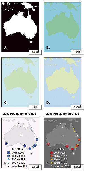
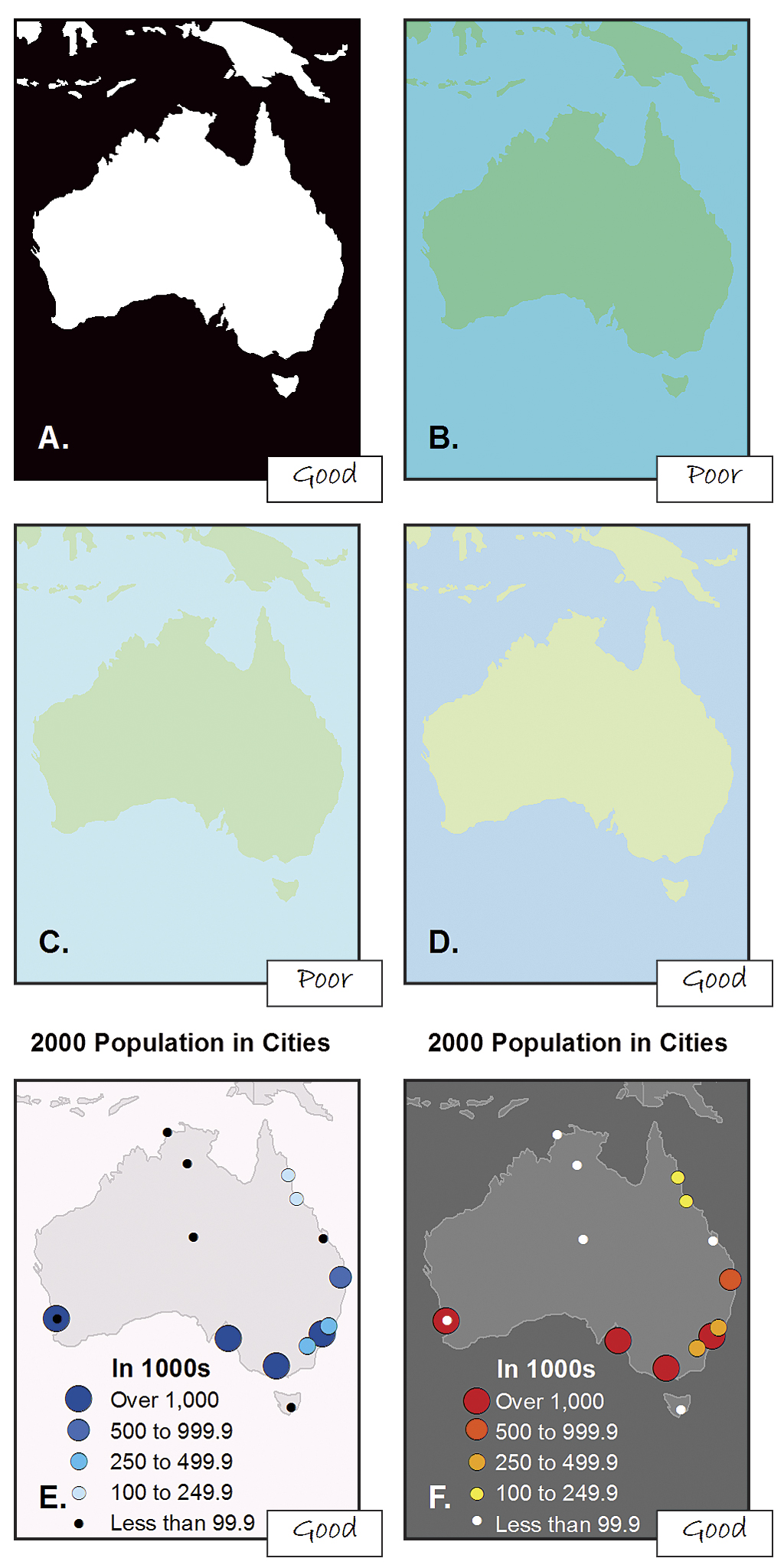
1) Visual Contrast

Visual contrast relates how map features and page elements contrast with each other and their background. To understand this principle at work, consider your inability to see well in a dark environment. Your eyes are not receiving much reflected light, so there is little visual contrast between the objects in your field of view and you cannot easily distinguish objects from one another or from their surroundings. Increase illumination, and you are now able to distinguish features from the background. However, the features will still need to be large enough to be seen and understood so that your mind can decipher what your eyes are detecting.
The concept of visual contrast also applies in cartography (Figure 1). A well-designed map with a high degree of visual contrast can result in a crisp, clean, sharp-looking map. The higher the contrast between features, the more some features will stand out (usually features that are darker or brighter). Conversely, a map that has low visual contrast can be used to promote a more subtle impression. Features that have less contrast appear to belong together.

Figure 2. Symbols (A) and text (C) that are too small are illegible. Appropriately sized symbols (B) and text (D) can be easily distinguished and read. Using familiar geometric icons, such as an airplane for airports (E), helps readers immediately understand the meaning of the symbol. More complex symbols, such as a mortarboard for universities (F), need to be larger to be legible.

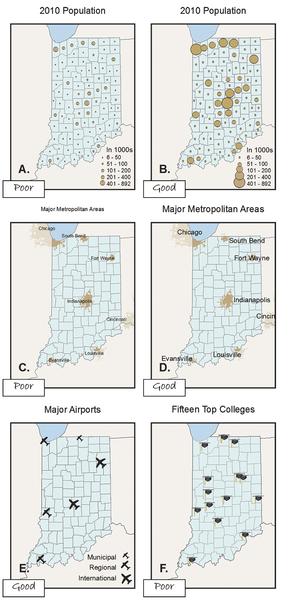
2) Legibility

Legibility is the ability to be seen and understood. Many people strive to make their map contents and page elements easily seen, but it is also important that they can be understood. Legibility depends on good decision making when selecting symbols. Choosing symbols that are familiar and are appropriate sizes results in symbols that are effortlessly seen and easily understood (Figure 2). Geometric symbols are easier to read at smaller sizes. More complex symbols require more space to be legible.
Visual contrast and legibility can also be used to promote the other design principles: figure-ground organization, hierarchical organization, and balance.

Figure 3. It is sometimes hard to tell what is the figure and what is the ground (A and B). Simply adding detail to the map (C) can help map readers distinguish the figure from the ground. Using a whitewash (D), feathering (E), or a drop shadow (F) can also help.

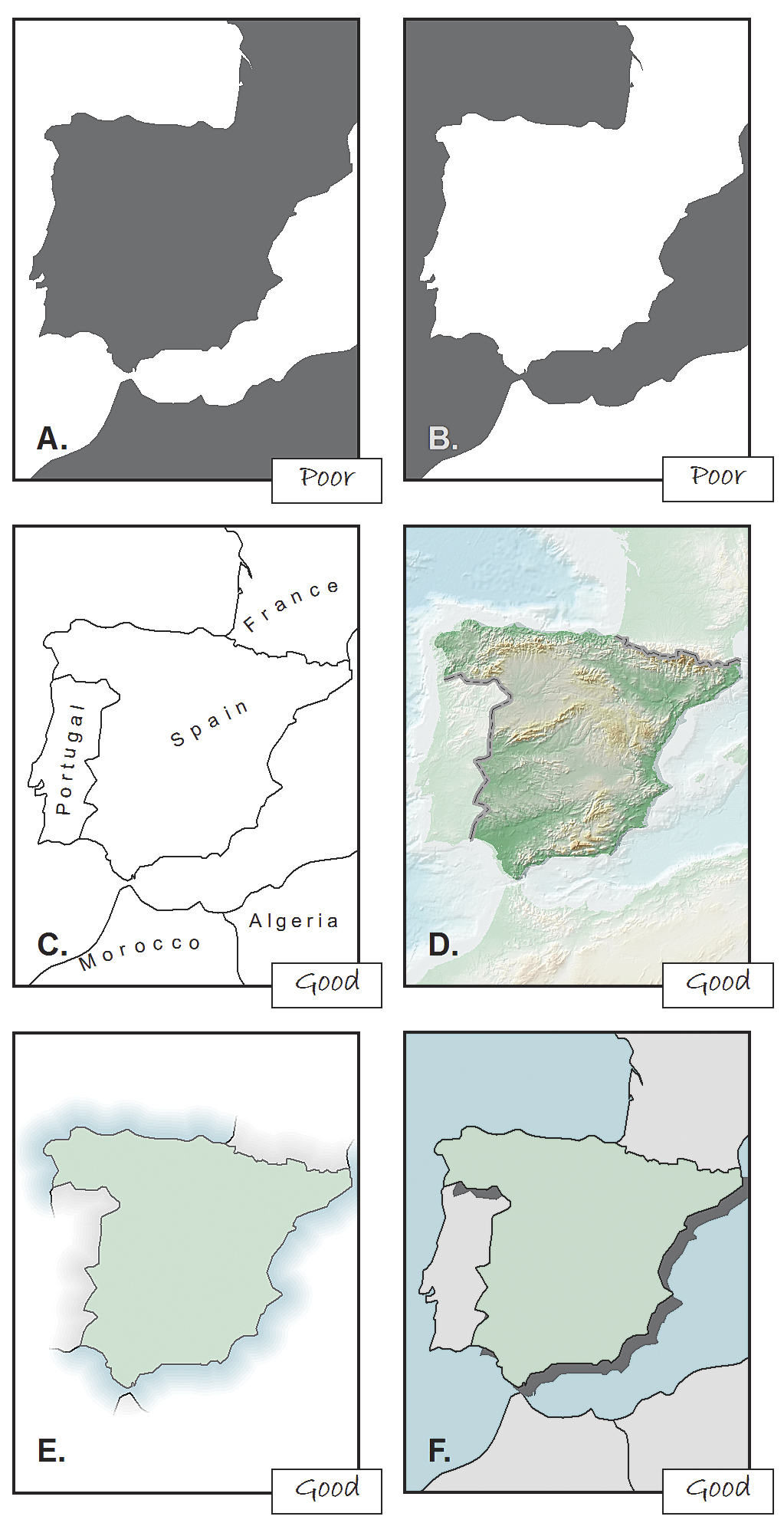
3) Figure-Ground Organization

Figure-ground organization is the spontaneous separation of the figure in the foreground from an amorphous background. Cartographers use this design principle to help map readers focus on a specific area of the map. There are many ways to promote figure-ground organization, such as adding detail to the map or using a whitewash, a drop shadow, or feathering.

Figure 4. When the symbols and labels are on the same visual plane (A), it is difficult for the map reader to distinguish among them and determine which are more important. For a general reference map (B), using different sizes for the text and symbols (e.g., city points and labels), different line styles (e.g., administrative boundaries), and different line widths (e.g., rivers) are some of the ways you can add hierarchy to the map. When mapping thematic data (C), the base information (e.g., county boundaries and county seats) should be kept to a minimum so that the theme (e.g., soils) is at the highest visual level in the hierarchy.

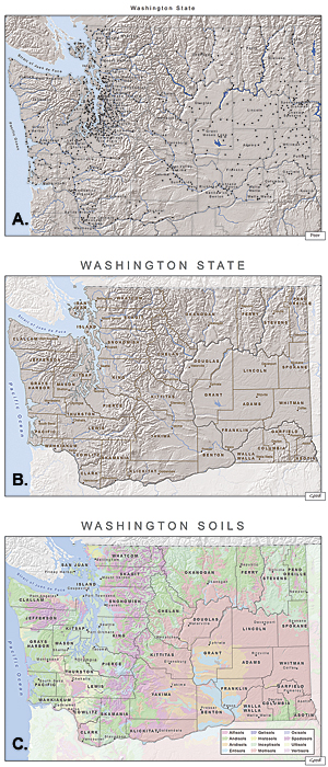
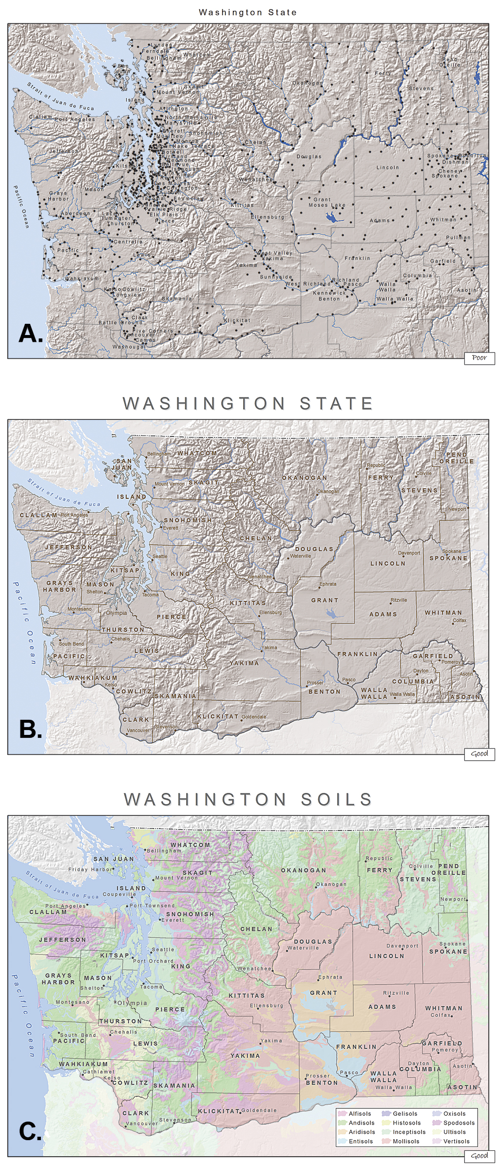
4) Hierarchical Organization

As noted in Elements of Cartography, Sixth Edition, one of the major objectives in mapmaking is to "separate meaningful characteristics and to portray likenesses, differences, and interrelationships." The internal graphic structuring of the map (and, more generally, the page layout) is fundamental to helping people read your map. You can think of a hierarchy as the visual separation of your map into layers of information. Some types of features will be seen as more important than other kinds of features, and some features will seem more important than other features of the same type. Some page elements (e.g., the map) will seem more important than others (e.g., the title or legend).
This visual layering of information within the map and on the page helps readers focus on what is important and lets them identify patterns. The hierarchical organization of reference maps (those that show the location of a variety of physical and cultural features, such as terrain, roads, boundaries, and settlements) works differently than for thematic maps (those that concentrate on the distribution of a single attribute or the relationship among several attributes). For reference maps, many features should be no more important than one another and so—visually—they should lie on essentially the same visual plane. In reference maps, hierarchy is usually more subtle and the map reader brings elements to the forefront by focusing attention on them. For thematic maps, the theme is more important than the base that provides geographic context.

Figure 5. Positioning heavier elements together can make the page look top-heavy (A) or bottom heavy (B). Centering the map slightly above center (C) ensures that it is in the most prominent position on the page. The position of elements can also cause the eye to move in a desired direction. In D, the title is the first thing read, followed by the locator map, then the map of Africa, and finally the legend.

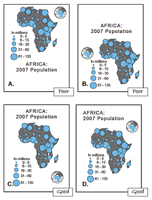
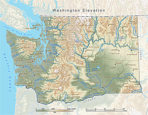
5) Balance

Balance involves the organization of the map and other elements on the page. A well-balanced map page results in an impression of equilibrium and harmony. You can also use balance in different ways to promote edginess or tension or create an impression that is more organic. Balance results from two primary factors: visual weight and visual direction. If you imagine that the center of your map page is balancing on a fulcrum, the factors that will tip the map in a particular direction include the relative location, shape, size, and subject matter of the elements on the page.
Together these five design principles have a significant impact on your map. How they are used will either draw the attention of map readers or potentially repel them. Giving careful thought to the design of your maps using these principles will help you to assure that your maps are ones people will want to look at!

Resources

These cartography textbooks provide more in-depth discussions of the design principles described in this article and how they are applied in cartography.
Dent, Borden D., Jeffrey S. Torguson, and Thomas H. Hodler. 2009. Cartography: Thematic Map Design, Sixth Edition, 207–222. Boston, MA: WCB-McGraw Hill.
Robinson, Arthur H., Joel L. Morrison, Phillip C. Muehrcke, A. Jon Kimerling, and Stephen C. Guptill. 1995. Elements of Cartography, Fifth Edition, 324–330. New York City, NY: John Wiley & Sons, Inc.
Slocum, Terry, Robert B. McMaster, Fritz C. Kessler, and Hugh H. Howard. 2009. Thematic Cartography and Geographic Visualization, Third Edition, 212–221. Upper Saddle River, NJ: Pearson Prentice Hall.

About the Author

Aileen Buckley is the lead of the Esri Mapping Center, an Esri website dedicated to helping users make professional-quality maps with ArcGIS. She has more than 25 years of experience in cartography and holds a doctorate in geography from Oregon State University. She has written and presented widely on cartography and GIS and is one of the authors of Map Use, Seventh Edition, published by Esri Press.